1. confusion_matrix (오분류표)

TN : 원래 값이 0인 값을 0으로 제대로 측정한 값 True Negative
FP : 원래 값은 0이지만 1로 잘못 예측한 값 False Positive
FN : 원래 값은 1이지만 0으로 잘못 예측한 값 False Negative
TP : 원래 값이 1인 값을 1로 제대로 측정한 값 True Positive
python 에서 confusion matrix 를 사용하기 위해 sklearn을 사용하였다.
from sklearn.metrics import confusion_matrix
confusion matrix 는 Accuracy, Precision, Recall(Sensitivity), Specificity, f1-score 등이 활용될 수 있다.
Accuracy = ( TN + TP ) / ( TN + FN + TP + FP ) : 전체 중 제대로 예측한 값
모델의 성능을 평가할 때 많이 쓰이는 값으로 모델이 얼마나 정확한지 나타내는 지표다.
Precision = TP / ( FP + TP ) : 1로 측정된 것 중에 실제로 1인 값
Recall = TP / ( TP + FN ) : 실제 1인 값들 중 1로 예측된 값
f1-score = 2 * Precision * Recall / ( Precision + Recall ) : 정밀도와 민감도의 조화평균
마냥 Accuracy가 높다고 좋은 모델이라고 할 수 없다. Accuracy가 0.8인 모델을 가지고 있는데 다른 모델은 전부 1로만 예측해버리는 모델이 있다고 가정해보자.
# 모두 1로 예측해버리는 FakeClassifier
class MyFakeClassifier(BaseEstimator):
    def fit(self, X, y):
        pass
    def predict(self, X):
        return np.zeros( (len(X), 1), dtype = 'bool')
digits = load_digits()

y = (digits.target == 7).astype('int')
X_train, X_test, y_train, y_test = train_test_split(digits.data, y, random_state = 42)
X_train.shape, X_test.shape, y_train.shape, y_test.shape

# ((1347, 64), (450, 64), (1347,), (450,))
clf = MyFakeClassifier()
clf.fit(X_train, y_train)
y_pred = clf.predict(X_test)

print(pd.Series(y_test).value_counts(), accuracy_score(y_test, y_pred), confusion_matrix(y_test, y_pred), sep = '\n')

# 0    409
# 1     41

# accuracy : 0.91

# confusion matrix
 [409   0]    TN  FP
 [ 41   0]    FN  TP
그럴경우 데이터가 100개중 91개가 1이라고 한다면 전부 1로 예측해버리는 모델의 Accuracy값은 0.91로 직접 튜닝을 통해 만든 Accuracy 보다 11% 더 높게 된다. 이럴 경우 Precision과 Recall 을 활용하여 모델을 평가하여야 한다.
precision = TP / ( FP + TP ) = 0 / ( 0 + 0 )
recall = TP / ( FN + TP ) = 0 / ( 41 + 0 )
accuracy 값은 높지만 Precision과 Recall 값은 정의할 수 없다.
이러한 문제들 때문에 Precision과 Recall 값의 중요성을 알 수 있다.
2. Precision과 Recall
기본적인 sigmoid function 을 사용하면 Thresholds 가 0.5 이다. 0.5 기준으로 0과 1을 분리하는 이진분류를 하게 되는데 이에 다음과 같은 문제가 발생할 수 있다. 병원에서 암세포 관련 검사를 받은 환자 중 암세포가 있다고 예측된 사람들 중 정상이 있다고 하는 것과 실제 암세포가 있는사람들 중 정상이라고 판단되는 것을 보면 전자의 경우 재검사 비용을 지불하고 큰 문제가 발생하지 않지만, 후자의 경우에는 암세포를 가진 사람은 암세포가 있다는 것을 모르기 때문에 큰 문제가 발생할 수 있다.
이런 경우에는 recall 값이 중요하게 된다. 하지만 recall 값을 올리기 위해 무분별하게 Thresholds 값을 낮추게 된다면 Precision 값이 낮아지고 Accuracy 값도 낮아지게 된다. 그러한 문제를 해결하기 위해 recall 과 Precision 의 조화평균인 f1 - score 값이 나오게 된다. f1 - score 값을 적절하게 측정하여 모델을 평가해야 된다.
예시를 보여주기 위하여 타이타닉 데이터를 활용하였다.
# 현재는 labeling 목적이 아니라 confusion matrix에 관해서만 다루고 있기 때문에 전처리 과정을 생략하고
# 변수값을 drop 하였습니다.
titanic.drop(['Name','Cabin', 'Ticket','Embarked'], axis = 1, inplace = True)
titanic.fillna(0, inplace = True)

#label encoding
le = LabelEncoder()
titanic['Sex'] = le.fit_transform(titanic['Sex'])


feature_cols = titanic.columns.difference(['Survived'])
y = titanic['Survived']
x = titanic[feature_cols]
x_train, x_test, y_train, y_test = train_test_split(x, y, random_state= 42)

x_train.shape, x_test.shape, y_train.shape, y_test.shape

# ((668, 7), (223, 7), (668,), (223,))


logit = LogisticRegression()
logit.fit(x_train, y_train)
y_pred = logit.predict(x_test)


def get_score(y_test, y_pred):
    confusion = confusion_matrix(y_test, y_pred)
    accuracy = accuracy_score(y_test, y_pred)
    precision = precision_score(y_test, y_pred)
    recall = recall_score(y_test, y_pred)
    print('confusion matrix')
    print(confusion)
    print('acc : {}, precision : {}, recall : {}'.format(accuracy, precision, recall))

get_score(y_test, y_pred)


# confusion matrix
# [[111  23]
# [ 28  61]]
# acc : 0.7713, precision : 0.7262, recall : 0.6854
precisions, recalls, thresholds = precision_recall_curve(y_pred, success)
# precision_recall_curve 는 precision, recall, threshold 값을 반환

# import matplotlib.pyplot as plt

plt.figure(figsize = (8,5))
plt.plot(thresholds, precisions[0:thresholds.shape[0]], linestyle = '--', label = 'precision' )
plt.plot(thresholds, recalls[0:thresholds.shape[0]], label = 'recall')
plt.xticks(np.arange(0,1.1,0.1))
plt.xlabel('Thresholds') ; plt.ylabel('Precision and Recall')
plt.legend()
plt.show()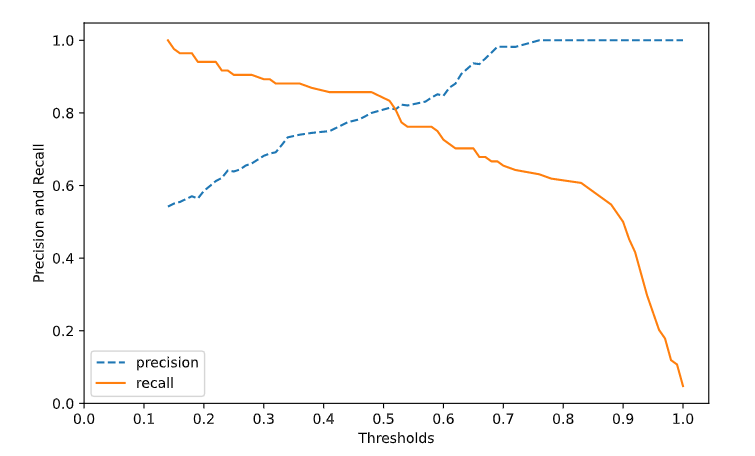
fprs, tprs, thresholds = roc_curve(y_test, success)

plt.plot(fprs, tprs, label = 'ROC')
plt.plot([0,1], [0,1], 'k--', label = 'Random')
plt.xlabel('FPR') ; plt.ylabel('TPR')
plt.legend()
plt.show()

Precision 과 recall 값을 잘 보고 적절한 Threshold 값을 찾아야한다.